How the 2021 reshuffling of NHL divisions will reduce traveling

I’m sure I’m not the only one out there who was very enthusiastic when the National Hockey League (NHL) unveiled its newly reshuffled divisions ahead of the 2021 season. I was secretly dreaming of an all-Canadian division for a long time, but never I thought that this dream could ever materialize. We’re entitled to expect electrifying hockey for the upcoming season, and some rivalries will certainly reach a higher, more emotional level, but what about the effect of this reshuffling on team traveling?
This post is the first of a series in which I will explore and explain different features of the
package tidynhl, a
personal project that is slowly but surely taking shape. The purpose of this package is to give
access to NHL data by facilitating the interaction with their open stats API, and to provide this
data on a ready-to-use and clean (or tidy) format.
Team schedules for the 2021 season
To begin, let’s get and print an excerpt of the NHL 2021 schedule with the tidy_schedules()
function.
# Load the packages
library(data.table)
library(tidynhl)

# Get the 2021 NHL schedule
nhl_schedule_2021 <- tidy_schedules(
  seasons_id = "20202021",
  playoffs = FALSE
)

# Print an excerpt
nhl_schedule_2021[]
#>      season_years season_type       game_datetime game_status             venue_name away_abbreviation away_score home_score home_abbreviation game_nbot game_shootout
#>   1:      2020-21     regular 2021-01-13 17:30:00       final     Wells Fargo Center               PIT          3          6               PHI         0         FALSE
#>   2:      2020-21     regular 2021-01-13 19:00:00       final       Scotiabank Arena               MTL          4          5               TOR         1         FALSE
#>   3:      2020-21     regular 2021-01-13 20:00:00       final           Amalie Arena               CHI          1          5               TBL         0         FALSE
#>   4:      2020-21     regular 2021-01-13 22:00:00       final           Rogers Place               VAN          5          3               EDM         0         FALSE
#>   5:      2020-21     regular 2021-01-13 22:30:00       final             Ball Arena               STL          4          1               COL         0         FALSE
#>  ---
#> 864:      2020-21     regular 2021-05-08 22:00:00   scheduled           Rogers Arena               CGY         NA         NA               VAN        NA            NA
#> 865:      2020-21     regular 2021-05-08 22:00:00   scheduled         T-Mobile Arena               STL         NA         NA               VGK        NA            NA
#> 866:      2020-21     regular 2021-05-08 22:00:00   scheduled         STAPLES Center               COL         NA         NA               LAK        NA            NA
#> 867:      2020-21     regular 2021-05-08 22:30:00   scheduled SAP Center at San Jose               ARI         NA         NA               SJS        NA            NA
#> 868:      2020-21     regular 2021-05-10 19:00:00   scheduled           Amalie Arena               DAL         NA         NA               TBL        NA            NA
Then, we will drop the useless columns and duplicate the rows in order to get a view of the schedule in the perspective of every teams. These steps will be done inside a function that will be reuse in a later section of the post.
# Define the create_teams_schedule() function
create_teams_schedule <- function(nhl_schedule) {

  teams_schedule <- rbindlist(list(
    nhl_schedule[, .(
      season = season_years,
      date = as.Date(game_datetime, tz = Sys.timezone()),
      status = "away",
      team = away_abbreviation,
      opponent = home_abbreviation
    )],
    nhl_schedule[, .(
      season = season_years,
      date = as.Date(game_datetime, tz = Sys.timezone()),
      status = "home",
      team = home_abbreviation,
      opponent = away_abbreviation
    )]
  ))

  teams_schedule[, venue := ifelse(status == "home", team, opponent)]

  setkey(teams_schedule, season, team, date)

  teams_schedule[]

}

# Call the function with the 2021 schedule
teams_schedule_2021 <- create_teams_schedule(nhl_schedule_2021)

# Print an excerpt
teams_schedule_2021[]
#>        season       date status team opponent venue
#>    1: 2020-21 2021-01-14   away  ANA      VGK   VGK
#>    2: 2020-21 2021-01-16   away  ANA      VGK   VGK
#>    3: 2020-21 2021-01-18   home  ANA      MIN   ANA
#>    4: 2020-21 2021-01-20   home  ANA      MIN   ANA
#>    5: 2020-21 2021-01-22   home  ANA      COL   ANA
#>   ---
#> 1732: 2020-21 2021-05-01   home  WSH      PIT   WSH
#> 1733: 2020-21 2021-05-03   away  WSH      NYR   NYR
#> 1734: 2020-21 2021-05-05   away  WSH      NYR   NYR
#> 1735: 2020-21 2021-05-07   home  WSH      PHI   WSH
#> 1736: 2020-21 2021-05-08   home  WSH      PHI   WSH
Feature engineering
The aim of this section is to create new features in the data representing the connection between successive games. Once again, this will be implemented through a reusable function that will create new columns indicating the date and location of the previous game. This function is created and called on our data in the code chunk below.
# Define the add_last_game() function
add_last_game <- function(teams_schedule) {

  teams_schedule[, `:=`(
    last_date = c(as.Date(NA), date[-.N]),
    last_venue = c(team, venue[-.N])
  ), .(season, team)]

}

# Call the function with the 2021 teams schedule
add_last_game(teams_schedule_2021)

# Print an excerpt
teams_schedule_2021[]
#>        season       date status team opponent venue  last_date last_venue
#>    1: 2020-21 2021-01-14   away  ANA      VGK   VGK       <NA>        ANA
#>    2: 2020-21 2021-01-16   away  ANA      VGK   VGK 2021-01-14        VGK
#>    3: 2020-21 2021-01-18   home  ANA      MIN   ANA 2021-01-16        VGK
#>    4: 2020-21 2021-01-20   home  ANA      MIN   ANA 2021-01-18        ANA
#>    5: 2020-21 2021-01-22   home  ANA      COL   ANA 2021-01-20        ANA
#>   ---
#> 1732: 2020-21 2021-05-01   home  WSH      PIT   WSH 2021-04-29        WSH
#> 1733: 2020-21 2021-05-03   away  WSH      NYR   NYR 2021-05-01        WSH
#> 1734: 2020-21 2021-05-05   away  WSH      NYR   NYR 2021-05-03        NYR
#> 1735: 2020-21 2021-05-07   home  WSH      PHI   WSH 2021-05-05        NYR
#> 1736: 2020-21 2021-05-08   home  WSH      PHI   WSH 2021-05-07        WSH
Then, we create another different table in which we will compute distances between any pair of team
venues. For the sake of simplicity, we’ll make the hypothesis that distances are calculated as the
crow flies. The geosphere package provides an
easy way to perform this with the distm() function.
In the chunk below, we will first retrieve metadata for each team (two of which are their venue’s
geographic coordinates and their actual division) using the tidy_teams_meta() function. We’ll then
compute a distance matrix as specified earlier and reorganize it as a table to make an eventual
merge easier.
# Load the package
library(geosphere)

# Get teams' metadata
teams_meta <- tidy_teams_meta()

# Print an excerpt
teams_meta[]
#>     team_abbreviation team_place      team_name        team_fullname team_shortname season_first_years conference_active_abbreviation conference_active_name division_active_abbreviation division_active_name venue_active_name venue_active_country venue_active_stateprovince venue_active_city     venue_active_tz venue_active_lat venue_active_long                                       logo_last_url
#>  1:               ANA    Anaheim          Ducks        Anaheim Ducks        Anaheim            1993-94                              W                Western                          WST           Honda West      Honda Center                  USA                         CA           Anaheim America/Los_Angeles         33.80778        -117.87667 https://assets.nhle.com/logos/nhl/svg/ANA_light.svg
#>  2:               ARI    Arizona        Coyotes      Arizona Coyotes        Arizona            2014-15                              W                Western                          WST           Honda West  Gila River Arena                  USA                         AZ          Glendale     America/Phoenix         33.53194        -112.26111 https://assets.nhle.com/logos/nhl/svg/ARI_light.svg
#>  3:               BOS     Boston         Bruins        Boston Bruins         Boston            1924-25                              E                Eastern                          EST      MassMutual East         TD Garden                  USA                         MA            Boston    America/New_York         42.36630         -71.06223 https://assets.nhle.com/logos/nhl/svg/BOS_light.svg
#>  4:               BUF    Buffalo         Sabres       Buffalo Sabres        Buffalo            1970-71                              E                Eastern                          EST      MassMutual East    KeyBank Center                  USA                         NY           Buffalo    America/New_York         42.87500         -78.87639 https://assets.nhle.com/logos/nhl/svg/BUF_light.svg
#>  5:               CAR   Carolina     Hurricanes  Carolina Hurricanes       Carolina            1997-98                              E                Eastern                          CEN     Discover Central         PNC Arena                  USA                         NC           Raleigh    America/New_York         35.80333         -78.72194 https://assets.nhle.com/logos/nhl/svg/CAR_light.svg
#> ---
#> 27:               TOR    Toronto    Maple Leafs  Toronto Maple Leafs        Toronto            1926-27                              E                Eastern                          NTH         Scotia North  Scotiabank Arena               Canada                         ON           Toronto     America/Toronto         43.64333         -79.37917 https://assets.nhle.com/logos/nhl/svg/TOR_light.svg
#> 28:               VAN  Vancouver        Canucks    Vancouver Canucks      Vancouver            1970-71                              W                Western                          NTH         Scotia North      Rogers Arena               Canada                         BC         Vancouver   America/Vancouver         49.27778        -123.10889 https://assets.nhle.com/logos/nhl/svg/VAN_light.svg
#> 29:               VGK      Vegas Golden Knights Vegas Golden Knights          Vegas            2017-18                              W                Western                          WST           Honda West    T-Mobile Arena                  USA                         NV         Las Vegas America/Los_Angeles         36.10278        -115.17833 https://assets.nhle.com/logos/nhl/svg/VGK_light.svg
#> 30:               WPG   Winnipeg           Jets        Winnipeg Jets       Winnipeg            2011-12                              W                Western                          NTH         Scotia North    Bell MTS Place               Canada                         MB          Winnipeg    America/Winnipeg         49.89278         -97.14361 https://assets.nhle.com/logos/nhl/svg/WPG_light.svg
#> 31:               WSH Washington       Capitals  Washington Capitals     Washington            1974-75                              E                Eastern                          EST      MassMutual East Capital One Arena                  USA                         DC        Washington    America/New_York         38.89806         -77.02083 https://assets.nhle.com/logos/nhl/svg/WSH_light.svg

# Compute a distance matrix in km
venues_matrix <- round(distm(teams_meta[, .(venue_active_long, venue_active_lat)]) / 1000L)

# Convert it to a table
teams_distances <- setDT(
  expand.grid(team = teams_meta[, team_abbreviation], opponent = teams_meta[, team_abbreviation])
)[, distance := as.integer(venues_matrix)]

# Print an excerpt
teams_distances[]
#>      team opponent distance
#>   1:  ANA      ANA        0
#>   2:  ARI      ANA      522
#>   3:  BOS      ANA     4161
#>   4:  BUF      ANA     3520
#>   5:  CAR      ANA     3566
#>  ---
#> 957:  TOR      WSH      563
#> 958:  VAN      WSH     3801
#> 959:  VGK      WSH     3364
#> 960:  WPG      WSH     2005
#> 961:  WSH      WSH        0
Travel analysis
Before going any further, we need to assume additional hypothesis regarding travel habits of teams. Of course, it’s impossible to have a perfect one-size-fits-all model, but I tried to rightly managed the required trade-off between simplicity and reality when designing the algorithm.
We will then assume the following assumptions:
- Each team is located home at the beginning of the season,
- Trips abroad follow the algorithm below.

To make sure it is well understood, we can apply the algorithm to the first few games of the Montreal Canadiens and analyze the result. For the first two weeks of the season, the resulting travels for the Habs are listed below:
January 13th 2021 game (MTL @ TOR)
- The team is in MTL when the season starts
⇒ Outcome: Traveling from MTL to TOR ✈️
January 16th 2021 game (MTL @ EDM)
- The team plays 2 successive away games (January 13th and 16th)
- Those games are not played against the same opponent (TOR and EDM)
- The closest opponent (TOR) is not further than 2,000 km away from MTL
- The team doesn’t have 3 off days between those games (only January 14th and 15th)
⇒ Outcome: Traveling from TOR to EDM ✈️
January 18th 2021 game (MTL @ EDM)
- The team plays 2 successive away games (January 16th and 18th)
- Those games are played against the same opponent (EDM)
⇒ Outcome: Not traveling 🏨
January 20th 2021 game (MTL @ VAN)
- The team plays 2 successive away games (January 18th and 20th)
- Those games are not played against the same opponent (EDM and VAN)
- The closest opponent (EDM) is further than 2,000 km away from MTL
- The team doesn’t have 5 off days between those games (only January 19th)
⇒ Outcome: Traveling from EDM to VAN ✈️
January 21st 2021 game (MTL @ VAN)
- The team plays 2 successive away games (January 20th and 21st)
- Those games are played against the same opponent (VAN)
⇒ Outcome: Not traveling 🏨
January 23rd 2021 game (MTL @ VAN)
- The team plays 2 successive away games (January 21st and 23rd)
- Those games are played against the same opponent (VAN)
⇒ Outcome: Not traveling 🏨
January 28th 2021 game (CGY @ MTL)
- The team doesn’t play 2 successive away games
⇒ Outcome: Traveling from VAN to MTL ✈️
We create a function implementing this algorithm and we apply it to every teams for the 2021 season.
# Define the create_teams_travels() function
create_teams_travels <- function(teams_schedule) {

  teams_travels <- teams_schedule[, rbindlist(mapply(
    FUN = function(team, venue, last_venue, off_days) {

      # Prevent names colliding
      TEAM <- team

      # No travel
      if (venue == last_venue) {
        return(NULL)
      }

      # Travel to next game
      if (is.na(off_days) | off_days < 3L | team %in% c(venue, last_venue)) {
        return(list(
          from = last_venue,
          to = venue
        ))
      }

      # Minimal distance from home
      distance <- teams_distances[team == TEAM & opponent %in% c(venue, last_venue), min(distance)]

      # Travel home + Travel to next game
      if (off_days >= 5L | (off_days >= 3L & distance <= 2000L)) {
        return(list(
          from = c(last_venue, team),
          to = c(team, venue)
        ))
      }

      # Travel to next game
      list(
        from = last_venue,
        to = venue
      )

    },
    team = team,
    venue = venue,
    last_venue = last_venue,
    off_days = date - last_date - 1L,
    SIMPLIFY = FALSE
  )), .(season, team)]

  # Add travel distances
  teams_travels[teams_distances, distance := distance, on = c(from = "team", to = "opponent")]

  # Output
  teams_travels[]

}

# Call the function with the 2021 teams schedule
teams_travels_2021 <- create_teams_travels(teams_schedule_2021)

# Print an excerpt
teams_travels_2021[]
#>       season team from  to distance
#>   1: 2020-21  ANA  ANA VGK      354
#>   2: 2020-21  ANA  VGK ANA      354
#>   3: 2020-21  ANA  ANA ARI      522
#>   4: 2020-21  ANA  ARI ANA      522
#>   5: 2020-21  ANA  ANA LAK       45
#>  ---
#> 744: 2020-21  WSH  BOS NYI      279
#> 745: 2020-21  WSH  NYI PHI      162
#> 746: 2020-21  WSH  PHI WSH      194
#> 747: 2020-21  WSH  WSH NYR      331
#> 748: 2020-21  WSH  NYR WSH      331
We could easily validate that the function gives the expected results for our previous specific example on the Canadiens.
teams_travels_2021[team == "MTL"][1:4]
#>     season team from  to distance
#> 1: 2020-21  MTL  MTL TOR      505
#> 2: 2020-21  MTL  TOR EDM     2714
#> 3: 2020-21  MTL  EDM VAN      819
#> 4: 2020-21  MTL  VAN MTL     3696
We then create a summary indicating the total distance on which each team will have to travel during the 2021 season. We also add the actual divisions for the matter of making comparisons among them.
# Define the create_teams_travel_summary() function
create_teams_travel_summary <- function(teams_travels, nhl_schedule) {

  # Create a summary table
  teams_travel_summary <- teams_travels[, .(
    nb = .N,
    km = sum(distance)
  ), .(season, team)]

  # Add the km per day variable
  nhl_season_days <- nhl_schedule[, .(
    season_years = season_years,
    game_date = as.Date(game_datetime, tz = Sys.timezone())
  )][, .(days = as.integer(max(game_date) - min(game_date) + 1L)), season_years]
  teams_travel_summary[nhl_season_days, days := days, on = c(season = "season_years")]
  teams_travel_summary[, km_per_day := km / days]

  # Add the divisions
  teams_travel_summary[teams_meta, division := division_active_name, on = c(team = "team_abbreviation")]

  # Output
  teams_travel_summary[]

}

# Call the function with 2021 teams travels
teams_travel_summary_2021 <- create_teams_travel_summary(teams_travels_2021, nhl_schedule_2021)

# Print an excerpt
teams_travel_summary_2021[]
#>      season team nb    km days km_per_day         division
#>  1: 2020-21  ANA 23 17275  118  146.39831       Honda West
#>  2: 2020-21  ARI 19 19110  118  161.94915       Honda West
#>  3: 2020-21  BOS 25  9012  118   76.37288  MassMutual East
#>  4: 2020-21  BUF 26 10483  118   88.83898  MassMutual East
#>  5: 2020-21  CAR 22 20457  118  173.36441 Discover Central
#> ---
#> 27: 2020-21  TOR 29 31852  118  269.93220     Scotia North
#> 28: 2020-21  VAN 22 33415  118  283.17797     Scotia North
#> 29: 2020-21  VGK 24 23275  118  197.24576       Honda West
#> 30: 2020-21  WPG 23 27515  118  233.17797     Scotia North
#> 31: 2020-21  WSH 25  7191  118   60.94068  MassMutual East
We now plot this data to facilitate its interpretation. The
ggplot2 and scales packages are
respectively used for creating the plot and customizing its format.
# Load the packages
library(ggplot2)
library(scales)

# Create the plot
ggplot(
  data = teams_travel_summary_2021,
  mapping = aes(
    x = km,
    y = reorder(as.factor(team), km),
    fill = division
  )
) +
  geom_col() +
  scale_x_continuous(
    labels = label_number(big.mark = ","),
    expand = expansion(mult = c(0, 0.05))
  ) +
  scale_fill_brewer(palette = "Set1") +
  labs(
    title = "Total traveling distance by team",
    subtitle = "2021 NHL season",
    x = "Distance (km)"
  )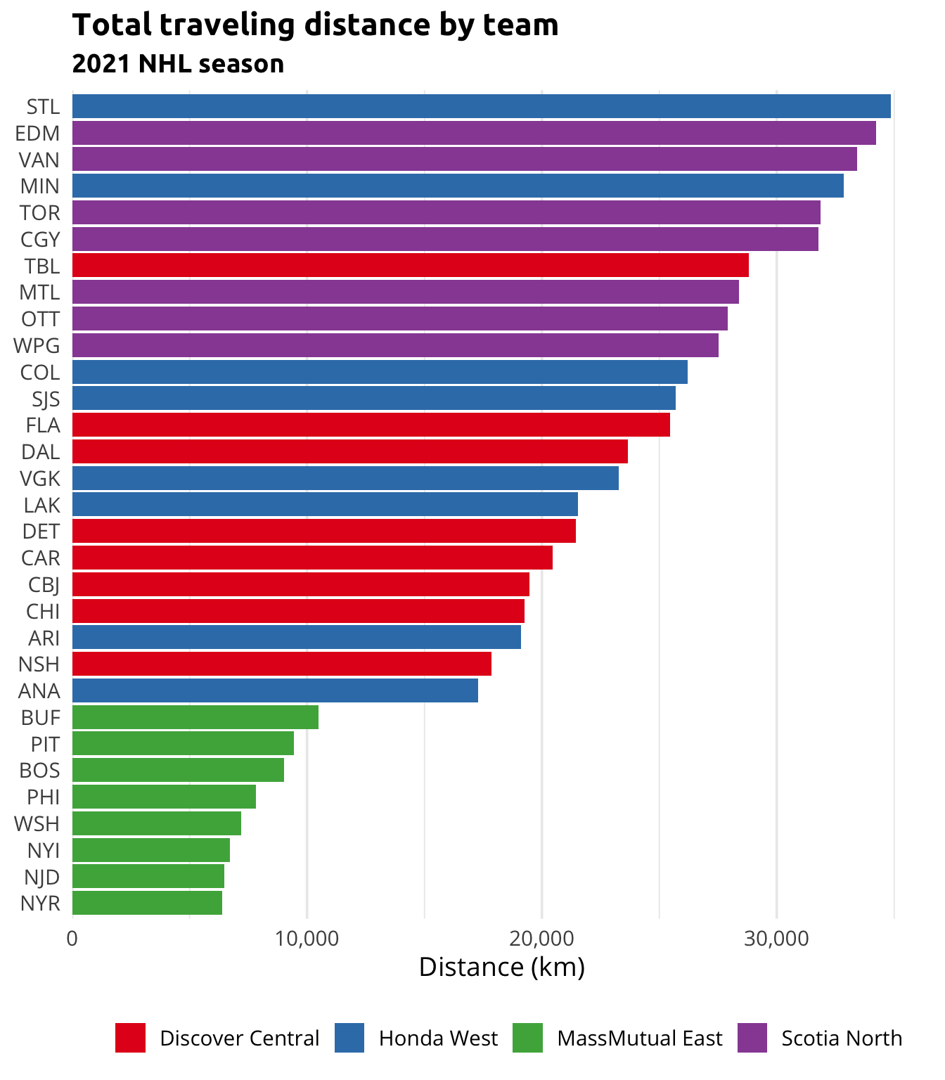
As one may probably have guessed right, the three teams in the New York Metropolitan Area (NYR, NYI and NJD) are those who will travel on the shortest distance for the season. Teams in the all-Canadian division are those that, in average, will travel on the greatest distance. However, one could observe that the distribution within this division is rather uniform, which is not the case for the Western division. Indeed, while the Anaheim Ducks will only need to travel a slight more than 17,000 km over the course of the season, the St. Louis Blues will accumulate just short of 35,000 km (more than twice 😱!) on the same period. We’ll see if that competitive advantage for the Ducks will prove enough to overcome their obvious lack of offensive skills…

One thing is sure, if the accumulated tiredness coming from traveling during the season is an important factor on player performances in playoffs, teams from the Eastern division will have a major headstart when playing other teams this spring.
Comparing with previous seasons
Although the absolute traveling distance of each team for the 2021 season is insightfull, it could also be interesting to look at the relative change induced by those new divisions and the new schedule patterns on each team. To do so, we will compare the 2021 season to seasons between 2013-14 (the last time the NHL reshuffled the divisions before this year) and 2019-20.
We reuse the functions defined in the last section one after the other. Then, we compute average metrics on those 7 seasons.
# Get the 2013-14 to 2019-20 NHL schedule
nhl_schedule_20132020 <- tidy_schedules(
  seasons_id = paste0(2013:2019, 2014:2020),
  playoffs = FALSE
)

# Replace PHX by ARI
nhl_schedule_20132020[away_abbreviation == "PHX", away_abbreviation := "ARI"]
nhl_schedule_20132020[home_abbreviation == "PHX", home_abbreviation := "ARI"]

# Create teams' schedule
teams_schedule_20132020 <- create_teams_schedule(nhl_schedule_20132020)

# Transform the data
add_last_game(teams_schedule_20132020)

# Create team's travels
teams_travels_20132020 <- create_teams_travels(teams_schedule_20132020)

# Create team's travels summary by season
teams_travel_summary_20132020 <- create_teams_travel_summary(teams_travels_20132020, nhl_schedule_20132020)

# Create team's travels summary
teams_travel_summary_20132020 <- teams_travel_summary_20132020[, .(
  season = "2013-20",
  km_avg = mean(km),
  km_per_day_avg = sum(km) / sum(days)
), .(team, division)]

# Print an excerpt
teams_travel_summary_20132020[]
#>     team         division  season   km_avg km_per_day_avg
#>  1:  ANA       Honda West 2013-20 71663.71       390.9945
#>  2:  ARI       Honda West 2013-20 77372.29       422.1403
#>  3:  BOS  MassMutual East 2013-20 63927.00       348.7833
#>  4:  BUF  MassMutual East 2013-20 55257.86       301.4848
#>  5:  CAR Discover Central 2013-20 62885.29       343.0998
#> ---
#> 27:  TOR     Scotia North 2013-20 56366.86       307.5355
#> 28:  VAN     Scotia North 2013-20 72433.43       395.1941
#> 29:  WPG     Scotia North 2013-20 71265.57       388.8223
#> 30:  WSH  MassMutual East 2013-20 57520.14       313.8277
#> 31:  VGK       Honda West 2013-20 69383.00       389.0636
To make sure we compare apples to apples, we will this time study the average daily traveling distance during the season. This metric ensures that the 2019-20 and 2021 seasons won’t skew the global picture because they were shortened due to the COVID-19 pandemic.
The following plot shows the observed decrease in average daily traveling distance by team for the 2021 season compared to the reference period. Results are sorted by relative decreasing.
# Create comparative summary
teams_travel_summary <- copy(teams_travel_summary_2021[, .(team, division, km_per_day_2021 = km_per_day)])
teams_travel_summary[teams_travel_summary_20132020, km_per_day_201320 := km_per_day_avg, on = .(team)]
teams_travel_summary[, km_per_day_cut := (km_per_day_2021 / km_per_day_201320) - 1]

# Create the plot
ggplot(
  data = teams_travel_summary,
  mapping = aes(
    y = reorder(as.factor(team), km_per_day_cut),
    fill = division
  )
) +
  geom_col(aes(x = km_per_day_2021), alpha = 1) +
  geom_col(aes(x = km_per_day_201320), alpha = 0.5) +
  geom_text(
    mapping = aes(
      x = km_per_day_2021,
      label = percent(km_per_day_cut, 1)
    ),
    nudge_x = 2,
    hjust = 0
  ) +
  scale_x_continuous(
    labels = label_number(big.mark = ","),
    expand = expansion(mult = c(0, 0.05))
  ) +
  scale_fill_brewer(palette = "Set1") +
  labs(
    title = "Traveling reduction by team",
    subtitle = "2021 vs 2013-14 to 2019-20 NHL seasons",
    x = "Average daily traveling distance (km)"
  )
There is no surprise in observing that the mini-series concept, in which two teams play successive games one agaist the other, does reduce the traveling distance for all and every teams. The big winners of this reshuffling are indisputably the Eastern division teams while those experiencing the most modest gains (yet still interesting) are mainly the Canadian teams. That being said, I forever am a mad Montreal Canadiens fan, and the most important thing of all for me is to see the Leafs (agin and again) proudly sitting in the last position of whatever ranking there is 😁.
Conclusion
Even though this post highlighted the traveling asymmetries created by the reshuffling of the NHL divisions, it still remains difficult to predict wether all of this will have a significant impact on the ice or not. The season promise to offer its share of unpredictable surprises, with some of them having probably even greater consequences at the end. Moreover, it’s important to remember that the schedule presented in this post is up-to-date as of today, but is very likely to change with little notice with COVID-19 local outbreaks. After all, there is not much we can do more than to wait and see, and of course, enjoy the show!

J.P. Le Cavalier
Data Scientist / Actuary
I consider myself as a hybrid between an actuary and a data scientist. I like to make things the right way.